Advanced SQL: Window Functions, CTEs, and Query Optimization

You can write basic CRUD. You know how to JOIN a table and filter with WHERE. You’ve even indexed your foreign keys.

But when your data hits the millions of rows, and your product manager asks for complex analytical reports—like running totals, year-over-year growth, or finding the top N users per category—basic SQL starts to break down. You end up with messy nested subqueries, glacially slow execution times, and logic that belongs in application code.

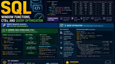
Welcome to the big leagues. Advanced SQL is about telling the database exactly what you want in a way the query optimizer can execute at lightning speed. Here is your guide to the three pillars of advanced SQL: Window Functions, CTEs, and Query Optimization.

Pillar 1: Window Functions (The Superpower)

If there is one skill that separates intermediate SQL developers from advanced ones, it's window functions.

A GROUP BY squashes multiple rows into a single output row. A window function performs a calculation across a set of rows related to the current row, without squashing them. The "window" is the frame of rows the function looks at.

The Anatomy of a Window Function

FUNCTION_NAME() OVER (
    PARTITION BY column_name  -- The "grouping"
    ORDER BY column_name      -- The sequence
    ROWS BETWEEN ... AND ...  -- The "frame"
)

1. Ranking: Finding the Top N per Category

Imagine you need the top 2 highest-paid employees in each department. You can't just do ORDER BY salary DESC LIMIT 2 because that limits the whole query.

SELECT 
    department,
    employee_name,
    salary,
    RANK() OVER (PARTITION BY department ORDER BY salary DESC) as dept_rank
FROM employees;

• RANK(): Leaves gaps if there are ties (1, 2, 2, 4).
• DENSE_RANK(): No gaps (1, 2, 2, 3).
• ROW_NUMBER(): Arbitrary sequential numbering, no ties allowed (1, 2, 3, 4).

2. Framing: Running Totals and Moving Averages

The ORDER BY in a window function defines a default frame: ROWS BETWEEN UNBOUNDED PRECEDING AND CURRENT ROW. This makes running totals trivial.

SELECT 
    order_date,
    daily_revenue,
    SUM(daily_revenue) OVER (ORDER BY order_date) as running_total,
    AVG(daily_revenue) OVER (ORDER BY order_date ROWS BETWEEN 6 PRECEDING AND CURRENT ROW) as 7_day_moving_avg
FROM daily_sales;

3. Lead and Lag: Comparing Rows

Want to calculate month-over-month growth? You need to compare a row to the previous row.

SELECT 
    month,
    revenue,
    LAG(revenue, 1) OVER (ORDER BY month) as prev_month_revenue,
    (revenue - LAG(revenue, 1) OVER (ORDER BY month)) / LAG(revenue, 1) OVER (ORDER BY month) as growth_rate
FROM monthly_sales;

graph LR
    A[Row 1] -->|LAG looks back| B[Row 2]
    B -->|LEAD looks forward| C[Row 3]

    style B fill:#4CAF50,color:#fff

⚠️ The Window Function Trap: Window functions are evaluated after WHERE, GROUP BY, and HAVING. You cannot put a window function in a WHERE clause. To filter by a rank, you must wrap the query in a CTE or Subquery.

Pillar 2: Common Table Expressions (CTEs)

CTEs (the WITH clause) are named temporary result sets that exist only for the duration of a single query. They were introduced to replace dense, unreadable nested subqueries.

1. CTEs for Readability

Compare the "old way" to the CTE way. The logic is identical, but the CTE reads top-to-bottom like procedural code.

The Messy Way:

SELECT d.name FROM (SELECT dept_id, COUNT(*) FROM employees GROUP BY dept_id HAVING COUNT(*) > 10) AS big_depts JOIN departments d ON big_depts.dept_id = d.id;

The Clean Way:

WITH BigDepartments AS (
    SELECT dept_id, COUNT(*) as emp_count
    FROM employees
    GROUP BY dept_id
    HAVING COUNT(*) > 10
)
SELECT d.name 
FROM BigDepartments bd
JOIN departments d ON bd.dept_id = d.id;

2. Recursive CTEs: Hierarchical Data

Recursive CTEs are a mind-bending but incredibly powerful tool for traversing trees or graphs (like org charts, file systems, or bill of materials).

A recursive CTE has a base case (the anchor) and a recursive step that references itself.

WITH RECURSIVE OrgChart AS (
    -- Anchor: Find the CEO
    SELECT id, name, manager_id, 1 as level
    FROM employees
    WHERE manager_id IS NULL

    UNION ALL

    -- Recursive Step: Find people managed by the previous level
    SELECT e.id, e.name, e.manager_id, oc.level + 1
    FROM employees e
    JOIN OrgChart oc ON e.manager_id = oc.id
)
SELECT * FROM OrgChart ORDER BY level;

3. The "Optimization Fence" Pro-Tip (Postgres)

In PostgreSQL, CTEs act as "optimization fences." The database materializes the CTE in memory before running the main query. * Good for: Caching an expensive calculation used multiple times in the main query. * Bad for: Pushing down WHERE clauses. If you filter the main query, Postgres can't push that filter into the CTE. (Note: Postgres 12+ changed this to inline non-recursive CTEs by default, but you can force the fence using WITH MATERIALIZED).

Pillar 3: Query Optimization

Writing a query that returns the right data is 50% of the job. Writing one that returns it in milliseconds is the other 50%.

1. Sargability: The Enemy of Indexes

Sargable stands for "Search Argument Able." If your WHERE clause is not sargable, the database cannot use an index; it must scan every single row.

❌ Non-Sargable (Index Ignored):

-- Wrapping the column in a function breaks the index
WHERE YEAR(created_at) = 2023
WHERE LOWER(email) = 'test@example.com'
WHERE salary + 1000 > 50000

✅ Sargable (Index Used):

-- Keep the column isolated on one side of the operator
WHERE created_at >= '2023-01-01' AND created_at < '2024-01-01'
WHERE email = 'test@example.com' -- Use case-insensitive collation instead
WHERE salary > 49000

2. SELECT * is a Performance Killer

• Network I/O: Pulling massive TEXT or JSONB columns when you only need an ID wastes bandwidth.
• Covering Indexes: If you have an index on (user_id, status), and you SELECT user_id, status, Postgres can satisfy the query entirely from the index (Index Only Scan). If you SELECT *, the database is forced to look up the actual row on disk (Heap Fetch).

3. The N+1 Problem in SQL (Correlated Subqueries)

A correlated subquery is one that references a column from the outer query. It looks clean, but it executes the inner query once for every row in the outer query.

❌ The N+1 Subquery:

SELECT e.name, 
       (SELECT d.name FROM departments d WHERE d.id = e.dept_id) as dept_name
FROM employees e;
-- If you have 10,000 employees, this runs the department query 10,000 times.

✅ The JOIN Solution:

SELECT e.name, d.name as dept_name
FROM employees e
JOIN departments d ON e.dept_id = d.id;
-- The optimizer evaluates this in one pass.

4. Learn to Read EXPLAIN ANALYZE

EXPLAIN shows the plan. ANALYZE actually runs the query and shows the actual time.

Look out for these red flags in your execution plan: 1. Seq Scan (Sequential Scan) on large tables: This means an index is missing or your query isn't sargable. 2. Nested Loop with a huge outer row estimate: Often indicates a missing index on the join key of the inner table. 3. High "actual time" on a single node: That's your bottleneck. Focus your optimization there.

graph TD
    A[Slow Query] --> B[Run EXPLAIN ANALYZE]
    B --> C{Find the Bottleneck Node}
    C -->|Seq Scan on big table| D[Add Index / Fix Sargability]
    C -->|Nested Loop| E[Add Index on Join Column]
    C -->|Hash Aggregate memory spill| F[Increase work_mem or Group By earlier]
    D --> G[Re-run EXPLAIN ANALYZE]
    E --> G
    F --> G

Conclusion

Advanced SQL is a different paradigm from basic CRUD. It requires you to think in sets, understand the order of execution (FROM -> WHERE -> GROUP BY -> HAVING -> SELECT -> ORDER BY), and empathize with the query optimizer.

Next time you write a query: 1. Use a CTE to make it readable. 2. Use a Window Function instead of bringing the data into Python/Pandas to calculate ranks or running totals. 3. Ensure your WHERE clauses are Sargable so your indexes actually fire.

Master these three pillars, and you won't just write queries that work—you'll write queries that scale.