
You just launched your new feature, and the dashboard is loading in 10 seconds. You check the logs, find the culprit query, and slap an index on the column in the WHERE clause. Boom. The query now takes 5 milliseconds.
You’ve just solved the symptom, but you might have created a new disease.
Indexes are the most powerful tool in a database administrator's arsenal for read performance, but they come with a heavy tax on writes and storage. Throwing indexes at a database without a strategy leads to bloated tables, slow inserts, and queries that still aren't fast enough.
In this guide, we’ll move beyond "add an index to slow columns" and explore the architectural strategies required to build high-performance, scalable databases.
The Anatomy of an Index: Why B-Trees Matter
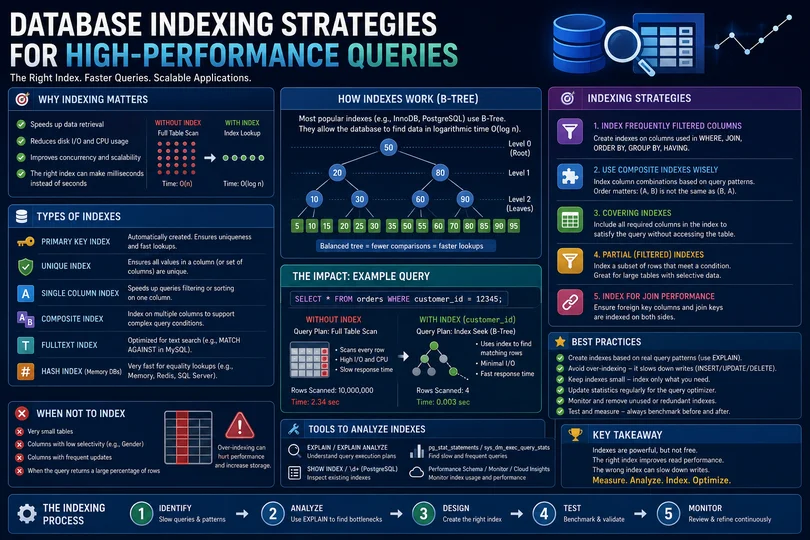
Before we strategize, we must understand how databases find data. Without an index, the database must perform a Full Table Scan—reading every single row from disk to find a match. It’s like reading a textbook from page 1 to find a specific keyword.
Most relational databases (Postgres, MySQL) use B-Tree (Balanced Tree) indexes by default. A B-Tree keeps data sorted and allows the database to traverse the tree in O(log N) time, turning a search of millions of rows into just 3-4 disk reads.
graph TD
    Root["Root: 40"] --> Left["Left Node: 10-20"]
    Root --> Right["Right Node: 50-70"]
    Left --> L1["Leaf: 5, 8"]
    Left --> L2["Leaf: 12, 15, 20"]
    Right --> R1["Leaf: 45, 50"]
    Right --> R2["Leaf: 60, 70, 85"]

    style Root fill:#f96,stroke:#333,stroke-width:2px
    style Left fill:#ff9,stroke:#333,stroke-width:2px
    style Right fill:#ff9,stroke:#333,stroke-width:2px
Strategy 1: The Cardinality Rule (Not All Columns Are Equal)
Cardinality refers to the number of unique values in a column. Indexes only work well when they help the database filter out the vast majority of rows.
- High Cardinality: Emails, UUIDs, Usernames (almost every row is unique). Excellent for indexing.
- Low Cardinality: Gender, Boolean flags (e.g.,
is_active). Useful when a queried value is rare, or as part of a partial/composite index.
If you index a boolean flag is_active where 99% of users are active, the database might just decide to do a Full Table Scan anyway, because reading the index + fetching the rows is actually more work than just reading the whole table.
🧠 Rule of Thumb: Measure selectivity for your actual predicates. There is no universal percentage cutoff: ordering, covering columns, row width, caching, and access cost also matter.
Strategy 2: Composite Indexes & The Left-Prefix Rule
The most common mistake developers make is creating single-column indexes for queries that filter by multiple columns.
Imagine this query:
SELECT * FROM orders
WHERE user_id = 123 AND status = 'shipped';
Separate indexes:
CREATE INDEX idx_user ON orders(user_id);
CREATE INDEX idx_status ON orders(status);
PostgreSQL can combine separate indexes using bitmap scans. A composite index can still be better for a frequent combined predicate or ordering; compare plans for your workload.
An alternative: Create a Composite Index.
CREATE INDEX idx_user_status ON orders(user_id, status);
The Left-Prefix Rule (Crucial)
A composite index is like a phonebook. A phonebook is sorted by Last Name, then First Name. * If you search for "Smith, John," the phonebook is blazing fast. * If you search for "Last Name = Smith," the phonebook is fast. * If you search for "First Name = John" (skipping the last name), the phonebook is completely useless. You must read the whole book.
The same applies to composite indexes. INDEX(A, B, C) can be used for:
✅ WHERE A = 1
✅ WHERE A = 1 AND B = 2
✅ WHERE A = 1 AND B = 2 AND C = 3
Queries on B or C alone may still use the index, but can scan more of it. PostgreSQL can also use skip scans in suitable cases. Choose column order for equality/range conditions, ordering, and common query prefixes, rather than always placing the highest-cardinality column first.
Strategy 3: Covering Indexes (The Ultimate Performance Hack)
When a database finds a match in the index, it usually has to do a Heap Fetch—jumping to the actual table row on disk to get the rest of the columns requested in the SELECT clause. Heap fetches are expensive I/O operations.
A Covering Index includes all the columns the query needs, making an index-only scan possible. In PostgreSQL, heap visibility checks may still require table access.
-- The query we want to optimize
SELECT user_id, status, created_at
FROM orders
WHERE user_id = 123;
We can use the INCLUDE clause (in Postgres/SQL Server) to store the data in the leaf nodes of the index without affecting the sorting tree:
-- Postgres syntax for a Covering Index
CREATE INDEX idx_user_covered
ON orders(user_id)
INCLUDE (status, created_at);
Measure heap fetches and buffer activity with EXPLAIN (ANALYZE, BUFFERS) to see whether the covering index actually reduces table access.
Strategy 4: Partial Indexes (Saving Space & Time)
Often, you only query a specific subset of your data. For example, an orders table might have millions of rows, but your dashboard only queries orders that are currently pending.
SELECT * FROM orders WHERE status = 'pending';
Indexing the entire table wastes disk space and slows down writes for all the completed and cancelled orders you don't care about.
A Partial Index only indexes rows that meet a specific condition.
-- Postgres syntax
CREATE INDEX idx_pending_orders
ON orders(status)
WHERE status = 'pending';
This can be smaller when pending orders are a small subset. Changes entering or leaving that subset still require index maintenance, and predicates must be evaluated.
Strategy 5: Specialized Index Types
B-Trees aren't the only tool in the shed. Depending on your data, other index structures are vastly superior:
- Hash Indexes: Only for exact equality (
=) checks. They cannot do range queries (>,<); size and speed depend on data and workload. Good for session IDs. - BRIN (Block Range Indexes): Used for massive tables with naturally sorted data (like timestamps in time-series data). Instead of indexing every row, it notes the "min" and "max" values of entire disk blocks. It's incredibly tiny and fast for chronological queries.
- GIN (Generalized Inverted Index): The standard for Full-Text Search and JSONB columns. If you need to search for a specific key inside a JSON payload, you need a GIN index.
sql -- Indexing JSONB in Postgres CREATE INDEX idx_metadata ON products USING GIN (metadata_jsonb); - Bitmap Indexes: Used in data warehousing (Oracle Database) for low-cardinality columns. Not typically used in OLTP databases like Postgres/MySQL.
The Write Penalty: Why You Must Be Ruthless
Indexes add write and storage costs, but not every change updates every index. PostgreSQL HOT updates can avoid index updates when eligible, and dead index entries may be cleaned later.
An insert into a table with six applicable indexes must maintain the table and those indexes; this is not a literal count of physical disk writes. Furthermore, indexes must remain balanced. High write volume can cause index bloat and page splits, degrading performance over time.
How to audit your indexes:
1. Find Duplicate or Redundant Indexes
An index on (A, B) may overlap one on (A), but compare uniqueness constraints, predicates, size, ordering, and workload before removing either.
2. Find Unused Indexes Postgres tracks index usage. Run this query periodically to find indexes that are taking up space but never being used:
SELECT schemaname, relname, indexrelname, idx_scan
FROM pg_stat_user_indexes
WHERE idx_scan = 0
ORDER BY pg_relation_size(indexrelid) DESC;
Zero scans are a review signal, not permission to drop an index. Check when statistics were reset, infrequent workloads, replicas, and constraint dependencies first.
Further reading: Combining indexes, Multicolumn indexes, Index-only scans.
Conclusion: Measure, Don't Guess
Indexing is a game of trade-offs. You are trading write performance and disk space for read performance.
Never add an index blindly. Always use EXPLAIN ANALYZE before and after your query to see exactly what the query planner is doing. Compare measured latency, rows, buffers, and write cost; no scan type is universally best. EXPLAIN ANALYZE executes the statement, so take care with writes.
Start with the cardinality of your data, build smart composite indexes, leverage covering indexes for hot paths, and ruthlessly prune unused indexes. Your database—and your users—will thank you.